 Who says math is not beautiful? Anyone who doubts the beauty in math must check out algebraic surfaces.
An implicit functions has the form:
where, 
For example, the implicit equation of the unit circle is 

An algebraic surface is described by an implicit function 

Here are some examples of algebraic surfaces plotted using Mayavi:
-

- Goursat: x^4+y^4+z^4+a(x^2+y^2+z^2)^2+b(x^2+y^2+z^2)+c=0
-

- Saddle: z = x^2 – y^2
-
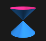
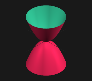
- Double cone: z^2 = Ax^2 + By^2
-
- Schwarz P: cos(x) + cos(y) + cos(z) = 0
-

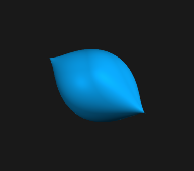
- Tear drop: x^2 + y^2 = (1-z)z^3
-

- Ding Dong: x^2 + y^2 = (1-z)z^2
I wrote a quick function called implicit_plot for plotting algebraic surfaces using Mayavi. The most important argument to the function is of course the expression string. It is probably not the best function, but the idea is to show how to plot implicit surfaces. The code snippet is included at the end of this post. Suggestions for improvement are always welcome.
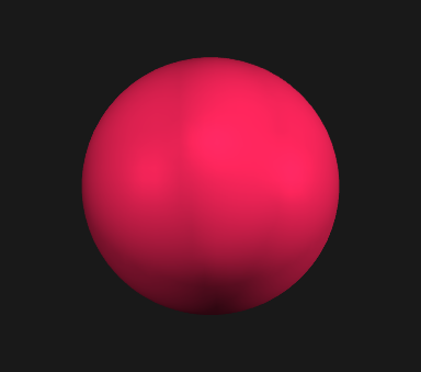
Let’s start with a simple sphere in three dimensional space, whose equation is 
implicit_plot like so (please note that it is assumed that mayavi has been imported in the script as mlab ):
import mayavi.mlab as mlab
figw = mlab.figure(1, bgcolor=(0.1, 0.1, 0.1), size=(400, 400))
implicit_plot('x**2 + y**2 + z**2 - {R:f}**2'.format(R=1), (-3, 3, -3, 3, -3, 3),
              fig_handle=figw, Nx=64, Ny=64, Nz=64, col_isurf=(0.0,0.2,0.8),
              opaque=True, ori_axis=False)
mlab.show()
Running the above code should render a sphere of unit radius in the given Mayavi figure window:
The equation 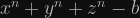


Here we study the various forms of surfaces represented by the above equation for 
![k \in [1, 2, \dots]](https://s0.wp.com/latex.php?latex=k+%5Cin+%5B1%2C+2%2C+%5Cdots%5D&bg=0f0f0f&fg=bbbbbb&s=1&c=20201002)

figw = mlab.figure(1, bgcolor=(0.97, 0.97, 0.97), size=(400, 400))
exponent = [2, 4, 6, 8, 10]
num_exponent = len(exponent)
col_isurf_arr = [(0.0,0.2,0.8), (0.2,0.5,0.4), (0.4,0.8,0.2),
                 (0.8,0.7,0.1), (1.0,0.2,0.0)] # colors
b = 100.0
for i, ex in enumerate(exponent):
    implicit_plot('x**{n} + y**{n} + z**{n} - {b}'.format(n=ex, b=b),
                  (-15, 15, -15, 15, -15, 15), fig_handle=figw,
                  Nx=64, Ny=64, Nz=64, col_isurf=col_isurf_arr[i],
                  opa_val=0.35+0.25*i/num_exponent, opaque=False, ori_axis=True)

mlab.show()
which produces the following output:
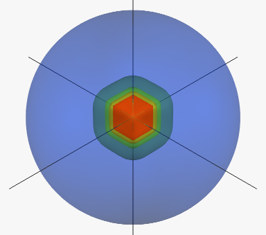
We can see that when 
figw = mlab.figure(1, bgcolor=(0.1, 0.1, 0.1), size=(400, 400))
implicit_plot('x**20 + y**20 + z**20 - 100',
              (-2, 2, -2, 2, -2, 2), col_osurf=(0.87,0.086,0.086),
              fig_handle=figw, opa_val=1.0, opaque=True, ori_axis=False)
mlab.show()
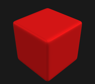
Next, we can study the surface transformations for odd values of 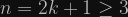
figw = mlab.figure(1, bgcolor=(0.1, 0.1, 0.1), size=(400, 400))
exponent = [2, 3, 5, 7, 9]
num_exponent = len(exponent)
col_isurf_arr = [(0.0,0.2,0.8), (0.2,0.5,0.4), (0.4,0.8,0.2),
                 (0.8,0.7,0.1), (1.0,0.2,0.0)] # colors
b = 100.0
for i, ex in enumerate(exponent):
    implicit_plot('x**{n} + y**{n} + z**{n} - {b}'.format(n=ex, b=b),
                  (-15, 15, -15, 15, -15, 15), fig_handle=figw,
                  Nx=64, Ny=64, Nz=64, col_isurf=col_isurf_arr[i],
                  opa_val=0.35+0.25*i/num_exponent, opaque=False, ori_axis=True)
mlab.show()
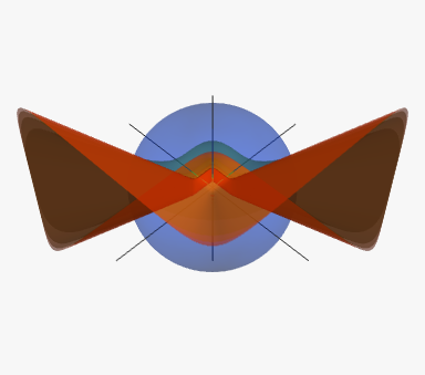
Multiple algebraic surfaces can be rendered by evaluating a product of the expressions. For example, the expression for 
![\prod_{i}^{N} \left[ (x - a_i)^2 + (y - b_i)^2 + (z - c_i)^2 - r_i^2 \right] = 0](https://s0.wp.com/latex.php?latex=%5Cprod_%7Bi%7D%5E%7BN%7D+%5Cleft%5B+%28x+-+a_i%29%5E2+%2B+%28y+-+b_i%29%5E2+%2B+%28z+-+c_i%29%5E2+-+r_i%5E2+%5Cright%5D+%3D+0&bg=0f0f0f&fg=bbbbbb&s=1&c=20201002)
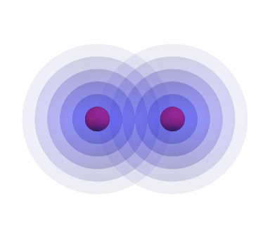
In the following example we render just two spheres:
figw = mlab.figure(1, bgcolor=(0.1, 0.1, 0.1), size=(400, 400))
# draw a base-plane
implicit_plot('(z + 0)', (-5, 5, -5, 5, -5, 5), fig_handle=figw,
             col_isurf=(0.1,0.1,0.1), opa_val=1.0, opaque=False, ori_axis=True)

# The two spheres
implicit_plot('(x**2 + y**2 + (z-1.414)**2 - 2)*((x-1.5)**2 + (y-1.5)**2 + (z-0.707)**2 - 0.5)',
              (-5, 5, -5, 5, -5, 5), fig_handle=figw, Nx=100, Ny=100, Nz=100,
              col_isurf=(0.87,0.086,0.086), opa_val=1.0, opaque=False, ori_axis=False)
mlab.show()
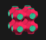
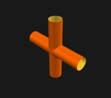
A 4-way tubing can be constructed by “adding” two cylinder surfaces together. As we saw above, two surfaces may be “added” together by multiplying the two surfaces equations. The equation for the 4-way tubing is thus 

figw = mlab.figure(1, bgcolor=(0.1, 0.1, 0.1), size=(400, 400))
implicit_plot('(x**2 + y**2 - 1)*(x**2 + z**2 - 1) - {a}'.format(a=0.005),
              (-5, 5, -5, 5, -5, 5), fig_handle=figw, Nx=201, Ny=201, Nz=201,
              col_isurf=(1.0,204./255,51./255), col_osurf=(1.0,102./255,0.0),
              opaque=True, ori_axis=False)
mlab.show()
Here are a few more examples of some interesting surfaces. The first one is known as the Zitrus surface whose equation is
(since the basic pattern of the code is same, we will just render the figure here)
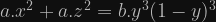
The next surface is Diabolo, which as the equation of the form
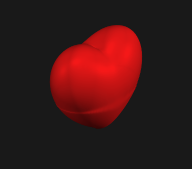
And finally, we render the well known Sweet surface whose expression is

Obviously, the algebraic surfaces are very beautiful, and there are really endless types of them for fun and study. The following extremely resourceful links can help the interested explorers of algebraic surfaces:
- Implicit function, Wikipedia
- List of complex and algebraic surfaces
- Algebraic surfaces Gallery, Hauser Herwig
- Algebraic surface, Wikipedia
- Algebraic surfaces, Gerhard Brunthaler
- Algebraic geometry, Wikipedia
- Algebraic variety, Wikipedia
- The Scientific Graphic Project, by David Hoffman, James Hoffman, Matthias Weber, et. al
- Surfaces at mathcurve
Here is the code snippet for the implicit_plot function
def implicit_plot(expr, ext_grid, fig_handle=None, Nx=101, Ny=101, Nz=101,
                 col_isurf=(50/255, 199/255, 152/255), col_osurf=(240/255,36/255,87/255),
                 opa_val=0.8, opaque=True, ori_axis=True, **kwargs):
    """Function to plot algebraic surfaces described by implicit equations in Mayavi

    Implicit functions are functions of the form

        `F(x,y,z) = c`

    where `c` is an arbitrary constant.

    Parameters
    ----------
    expr : string
        The expression `F(x,y,z) - c`; e.g. to plot a unit sphere, the `expr` will be `x**2 + y**2 + z**2 - 1`
    ext_grid : 6-tuple
        Tuple denoting the range of `x`, `y` and `z` for grid; it has the form - (xmin, xmax, ymin, ymax, zmin, zmax)
    fig_handle : figure handle (optional)
        If a mayavi figure object is passed, then the surface shall be added to the scene in the given figure. Then, it is the responsibility of the calling function to call mlab.show().
    Nx, Ny, Nz : Integers (optional, preferably odd integers)
        Number of points along each axis. It is recommended to use odd numbers to ensure the calculation of the function at the origin.
    col_isurf : 3-tuple (optional)
        color of inner surface, when double-layered surface is used. This is also the specified color for single-layered surface.
    col_osurf : 3-tuple (optional)
        color of outer surface
    opa_val : float (optional)
        Opacity value (alpha) to use for surface
    opaque : boolean (optional)
        Flag to specify whether the surface should be opaque or not
    ori_axis : boolean
        Flag to specify whether a central axis to draw or not

    """
    if fig_handle==None:  # create a new figure
        fig = mlab.figure(1,bgcolor=(0.97, 0.97, 0.97), fgcolor=(0, 0, 0), size=(800, 800))
    else:
        fig = fig_handle
    xl, xr, yl, yr, zl, zr = ext_grid
    x, y, z = np.mgrid[xl:xr:eval('{}j'.format(Nx)),
                       yl:yr:eval('{}j'.format(Ny)),
                       zl:zr:eval('{}j'.format(Nz))]
    scalars = eval(expr)
    src = mlab.pipeline.scalar_field(x, y, z, scalars)
    if opaque:
        delta = 1.e-5
        opa_val=1.0
    else:
        delta = 0.0
        #col_isurf = col_osurf
    # In order to render different colors to the two sides of the algebraic surface,
    # the function plots two contour3d surfaces at a "distance" of delta from the value
    # of the solution.
    # the second surface (contour3d) is only drawn if the algebraic surface is specified
    # to be opaque.
    cont1 = mlab.pipeline.iso_surface(src, color=col_isurf, contours=[0-delta],
                                      transparent=False, opacity=opa_val)
    cont1.compute_normals = False # for some reasons, setting this to true actually cause
                                  # more unevenness on the surface, instead of more smooth
    if opaque: # the outer surface is specular, the inner surface is not
        cont2 = mlab.pipeline.iso_surface(src, color=col_osurf, contours=[0+delta],
                                          transparent=False, opacity=opa_val)
        cont2.compute_normals = False
        cont1.actor.property.backface_culling = True
        cont2.actor.property.frontface_culling = True
        cont2.actor.property.specular = 0.2 #0.4 #0.8
        cont2.actor.property.specular_power = 55.0 #15.0
    else:  # make the surface (the only surface) specular
        cont1.actor.property.specular = 0.2 #0.4 #0.8
        cont1.actor.property.specular_power = 55.0 #15.0

    # Scene lights (4 lights are used)
    engine = mlab.get_engine()
    scene = engine.current_scene
    cam_light_azimuth = [78, -57, 0, 0]
    cam_light_elevation = [8, 8, 40, -60]
    cam_light_intensity = [0.72, 0.48, 0.60, 0.20]
    for i in range(4):
        camlight = scene.scene.light_manager.lights[i]
        camlight.activate = True
        camlight.azimuth = cam_light_azimuth[i]
        camlight.elevation = cam_light_elevation[i]
        camlight.intensity = cam_light_intensity[i]
    # axis through the origin
    if ori_axis:
        len_caxis = int(1.05*np.max(np.abs(np.array(ext_grid))))
        caxis = mlab.points3d(0.0, 0.0, 0.0, len_caxis, mode='axes',color=(0.15,0.15,0.15),
                              line_width=1.0, scale_factor=1.,opacity=1.0)
        caxis.actor.property.lighting = False
    # if no figure is passed, the function will create a figure.
    if fig_handle==None:
        # Setting camera
        cam = fig.scene.camera
        cam.elevation(-20)
        cam.zoom(1.0) # zoom should always be in the end.
        mlab.show()
Please note that the main block in the the above function is really the following three lines, which generates a scalar field on regular grid using the Mayavi pipleline, and then generates a zero-value isosurface:
scalars = eval(expr)
src = mlab.pipeline.scalar_field(x, y, z, scalars)
cont1 = mlab.pipeline.iso_surface(src, color=col_isurf, contours=[0],transparent=False, opacity=opa_val)
Hope you enjoyed the post.

Nice post. I’ve been trying to plot the crixxi surface (y^2 + z^2 – 1)^2 + (x^2 + y^2 – 1)^3 = 0 and I’m running aground on the singularities. Any thoughts on smoothing these out?
Thank you. You are right about it. I have found this type of problem before. However, I don’t think that I have a very good solution. Generally, to reduce the artifacts I add a very small value to the equation (i.e. I don’t try to solve for the zero set). For example, for the crixxi surface, I could generate the following figure (shown below) using the following code;
import mayavi.mlab as mlab
from iutils.plotutils.mayaviutils import implicit_plot

figw = mlab.figure(1, bgcolor=(0.1, 0.1, 0.1), size=(600, 600))

implicit_plot('(x**2 + y**2 - 1)**3 + (y**2 + z**2 - 1)**2 - {a}'.format(a=0.0003),
               (-1.2, 1.2, -1.2, 1.2, -1.5, 1.5), fig_handle=figw,
               Nx=251, Ny=251, Nz=251, opaque=False, opa_val=0.8, ori_axis=False)

mlab.show()
Rendered image:
Let me know if that helps, or if you come up with something better.
Thanks.
This is so amazing and beautiful.