Ambiguity function (AF) and its use in OTF analysis

The 2D Ambiguity Function (AF) and its relation to 1D Optical Transfer Function (OTF)

The Ambiguity Function (AF) is an useful tool for optical system analysis. This post is a basic introduction to AF, and how it can be useful for analyzing incoherent optical systems. We will see that the AF simultaneously contains all the OTFs associated with an rectangularly separable incoherent optical system with varying degree of defocus [2-4]. Thus by inspecting the AF of an optical system, one can easily predict the performance of the system in the presence of defocus. It has been used in the design of extended-depth-of-field cubic phase mask system.

NOTE:

This post was created using an IPython notebook. The most recent version of the IPython notebook can be found here.

To understand the basic theory, we shall consider a one-dimensional pupil function, which is defined as:

$(1) \hspace{40pt} P(x) = \begin{cases} 1 & \text{if } |x| \leq 1, \\ 0 & \text{if } |x| > 1, \end{cases}$

The *generalized pupil function* associated with $P(x)$ is the complex function $\mathcal{P}(x)$ given by the expression [1]:

$(2) \hspace{40pt} \mathcal{P}(x) = P(x)e^{jkW(x)}$

where $W(x)$ is the aberration function. Then, the amplitude PSF of an aberrated optical system is the Fraunhofer diffraction pattern (Fourier transform with the frequency variable $f_x$ equal to $x/\lambda z_i$ ) of the generalized pupil function, and the intensity PSF is the squared magnitude of the amplitude PSF [1]. Note that $z_i$ is the distance between the diffraction pattern/screen and the aperture/pupil.

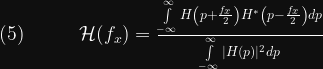
For the purpose of analyzing optical systems using the ambiguity function, it is convenient to separate the defocus term ( $W_{20}$ is the wavefront focus error coefficient [3]) from the rest of the aberration terms in the aberration function $W(x)$ :

$(3) \hspace{40pt} \begin{array}{rl} \mathcal{P}(x) &= P(x)e^{jkW(x)} \\ &= P(x)e^{jk(\tilde{W}(x) + W_{20}x^2)} \\ &= \mathcal{P}_o(x)e^{jkW_{20}x^2} \end{array}$

Since the amplitude PSF is the Fourier transform of the pupil function (see above), and the amplitude transfer function (ATF) is the Fourier transform of the amplitude PSF, the ATF is proportional to a scaled pupil function $\mathcal{P}$ . Specifically, the ATF $H(f_x)$ , is:

$(4) \hspace{40pt} H(f_x) = \mathcal{P}(\lambda z_i f_x)$

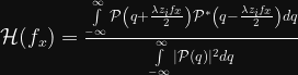
The (one dimensional) optical transfer function (OTF) is defined as the normalized autocorrelation of the ATF:

$(5) \hspace{40pt} \mathcal{H}(f_x) = \frac{\int\limits_{-\infty}^{\infty} H \left(p + \frac{f_x}{2}\right) H^* \left(p - \frac{f_x}{2} \right) dp}{\int\limits_{-\infty}^{\infty} |H(p)|^2 dp}$

$\hspace{50pt} \mathcal{H}(f_x) = \frac{\int\limits_{-\infty}^{\infty} \mathcal{P} \left(q + \frac{\lambda z_i f_x}{2}\right) \mathcal{P}^* \left(q - \frac{\lambda z_i f_x}{2} \right) dq} {\int\limits_{-\infty}^{\infty} |\mathcal{P}(q)|^2 dq}$

writing $u$ in place of $\lambda z_i f_x$ , we have

$\hspace{50pt} \mathcal{H}(u) = \frac{\int\limits_{-\infty}^{\infty} \mathcal{P} \left(q + \frac{u}{2}\right) \mathcal{P}^* \left(q - \frac{u}{2} \right) dq} {\int\limits_{-\infty}^{\infty} |\mathcal{P}(q)|^2 dq}$

$\hspace{50pt} \mathcal{H}(u) = \frac{\int\limits_{-\infty}^{\infty} \mathcal{P}_o\left(q + \frac{u}{2}\right) e^{jkW_{20}(q + u/2)^2} \mathcal{P}_o^* \left(q - \frac{u}{2} \right) e^{-jkW_{20}(q - u/2)^2} dq} {\int\limits_{-\infty}^{\infty} |\mathcal{P}_o(q)e^{jkW_{20}q^2}|^2 dq}$

$\hspace{50pt} \mathcal{H}(u) = \frac{\int\limits_{-\infty}^{\infty} \mathcal{P}_o\left(q + \frac{u}{2}\right) \mathcal{P}_o^* \left(q - \frac{u}{2} \right) e^{jkW_{20} [(q + u/2)^2 - (q - u/2)^2 ]} dq} {\int\limits_{-\infty}^{\infty} |P(q)|^2 dq}$

The simplified equation is written as follows:

$(6) \hspace{40pt} \mathcal{H}(u; W_{20}) = 0.5 \int\limits_{-\infty}^{\infty} \mathcal{P}_o\left(q + \frac{u}{2}\right) \mathcal{P}_o^* \left(q - \frac{u}{2} \right) e^{j 2\pi \left(\frac{2 W_{20}}{\lambda} \right)uq} dq$

The ambiguity function, which is used for radar analysis, is defined as the Fourier transform of the product $f(y + u/2) f^*(y - u/2)$ :

$(7) \hspace{40pt} A(u, y) = \int\limits_{-\infty}^{\infty}f\left(t + \frac{u}{2} \right) f^*\left(t - \frac{u}{2} \right)e^{j2\pi yt} dt$

Comparing the simplified expression of the aberrated OTF, $\mathcal{H}(u; W_{20})$ , and the ambiguity function, $A(u, y)$ , we see that:

$(8) \hspace{40pt} \mathcal{H}(u; W_{20}) = A \left(u, 2 u \frac{W_{20}}{\lambda} \right)$

This implies that the ambiguity function $A(u, y)$ associated with a base function $\mathcal{P}_o(u)$ contains the OTF $\mathcal{H}(u; W_{20})$ along the line $y = \frac{2 W_{20}}{\lambda} u$ (which has a slope $\tan (\phi) =\frac{2 W_{20}}{\lambda}$ , and passes through the origin in the $y-u$ plane as shown in the following figure.

Note:

1. The “base function” itself does not contain the defocus term, although it may contain other aberrations (see equation (3)).

2. Equation (6) is the “normalized autocorrelation” of the generalized pupil function, which implies that the maximum value of the function is 1. In equation (7) there is no explicit normalization and so the maximum value can be greater or less than 1. We must be mindful of this when comparing the AF to the OTF and prefer to chose appropriate amplitude for the base function $f(u)$ (as shown below).

In fact, the whole 2-D AF contains the OTFs $\mathcal{H}(u; W_{20})$ for various values of defocusing $W_{20}$ arranged in a polar fashion. Of special interest is the in-focus OTF for which $W_{20}=0$ and hence corresponds to the line along the “ $u$ ” axis. i.e. $\mathcal{H}(u; 0) = A(u,0)$

Example: Ambiguity function of a diffraction limited 1-D pupil.

If the only aberration is that of defocus, $\tilde{W}(x)=0$ in the expression for the generalized pupil function. Therefore the base-function which we consider is

$(9) \hspace{40pt} \mathcal{P}_o(x) = P(x) = \begin{cases} 1 & \text{if } |x| \leq 1, \\ 0 & \text{if } |x| > 1, \end{cases}$

First, we will consider the evaluation of the following integral of the general form:

$(10) \hspace{40pt} I(a, y) = \int\limits_{-\infty}^{\infty}f(t + a) f^*(t - a)e^{j2\pi yt} dt$

where, the function $f(t)$ is defined as:

$\hspace{50pt} f(t) = \begin{cases} A & \text{if } |t| \leq L, \\ 0 & \text{if } |t| > L, \end{cases}$

The following figure, which shows the regions of overlap between $f(t-a)$ and $f(t+a)$ (with $A=1$ ), is useful to understand the finite limites of the integral.

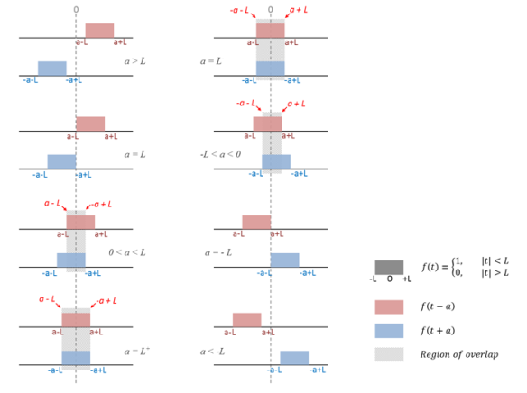
When $0 < a < L$ :

$\begin{array}{cl} I(a, y) &= \int\limits_{a-L}^{-a+L} A^2 e^{j2\pi yt} dt \\ &= A^2 \left| \frac{e^{j2\pi yt}}{j2\pi y} \right|_{a-L}^{-a+L} \\ &= A^2 \frac{1}{\pi y} \left[ \frac{e^{j2\pi (L-a)y} - e^{-j2\pi (L-a)y} }{2j} \right] \\ &= A^2 \frac{1}{\pi y} \sin{( 2\pi (L-a)y)} \\ &= 2(L-a)A^2 \frac{\sin{( 2\pi (L-a)y)}} {2\pi (L-a) y} \\ &= 2(L-a)A^2 \text{sinc}[2(L-a)y] \end{array}$

where, the $\text{sinc}$ function used above is the normalized $\text{sinc}$ that is defined as $\text{sinc}(x)=sin(\pi x)/(\pi x)$

When $-L < a \leq 0$ :

$\begin{array}{cl} I(a, y) &= \int\limits_{-a-L}^{a+L} A^2 e^{j2\pi yt} dt \\ &= A^2 \left| \frac{e^{j2\pi yt}}{j2\pi y} \right|_{-a-L}^{a+L} \\ &= A^2 \frac{1}{\pi y} \left[ \frac{e^{j2\pi (L+a)y} - e^{-j2\pi (L+a)y} }{2j} \right] \\ &= A^2 \frac{1}{\pi y} \sin{( 2\pi (L+a)y)} \\ &= 2(L+a)A^2 \frac{\sin{( 2\pi (L+a)y)}} {2\pi (L+a) y} \\ &= 2(L+a)A^2 \text{sinc}[2(L+a)y] \end{array}$

Note that we really didn’t have to break the integral into two parts. Instead we could just evaluate the integral between the limits $-(L - |a|)$ and $(L - |a|)$ .

We can combine the two cases and write the equation more compactly as:

$(11) \hspace{40pt} \begin{array}{ll} I(a, y) &= \int\limits_{-\infty}^{\infty}f(t + a) f^*(t - a)e^{j2\pi yt} dt \\ &= 2(L - |a|)A^2 \text{sinc}[2(L - |a|)y], \end{array} \,\,\, \text{for } |a| \leq L$

In our example, for which the base function is $\mathcal{P}_o = P(u)$ , the parameters $a=u/2$ , $A=\frac{1}{\sqrt{2}}$ (so that the maximum value is 1) and $L=1$ . We can now write:

$(12) \hspace{40pt} \begin{array}{ll} A(u, y) &= \int\limits_{-\infty}^{\infty}\mathcal{P}_o(t + a) \mathcal{P}_o^*(t - a)e^{j2\pi yt} dt \\ &= \left(1 - \frac{|u|}{2}\right)\text{sinc} \left[y(2 - |u|)\right] \end{array}$

Now, from equation (8) we have $\mathcal{H}(u; W_{20}) = A(u, 2 u W_{20}/\lambda)$ . Therefore we can write the expression for the OTF directly from the AF.

$(13) \hspace{40pt} \mathcal{H}(u; W_{20}) = \left(1 - \frac{|u|}{2} \right) \text{sinc} \left[ \frac{2 u W_{20}}{\lambda} (2 - |u|) \right]$

Note:

In [2], the authors have used the *un-normalized* $\text{sinc}$ function that is defined as $\text{sinc}(x)=\sin(x)/x$ . Hence, there is an “extra” $\pi$ within the $\text{sinc}$ function in their paper. We use the normalized definition $\text{sinc}$ as it is used in [1], and in Numpy.

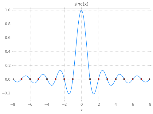
The figure below (after the code block) shows the function $\text{sinc}(x)$ for $x\in[-8,8]$ . It can be seen in figure that roots of the (normalized) $\text{sinc}$ function occurs at $x=n, n\neq 0, n \in \mathbb{Z}$ . Therefore the zero value loci for the AF associated with the one-dimensional rectangular pupil are found by equating $y(2 - |u|)=n$ .

from __future__ import print_function, division
import numpy as np
import scipy as sp
import matplotlib.cm as cm
import matplotlib.pyplot as plt
from IPython.display import Image
%matplotlib inline

x = np.linspace(-8, 8, 150)
y = np.sinc(x)
fig, ax = plt.subplots(1,1)
ax.plot(x, y, label='$sinc(x)$')
ax.set_ylim(-0.3, 1.02)
ax.set_xlim(-8, 8)
ax.set_xlabel('x')
ax.set_title('sinc(x)', y=1.02)
rootsx = range(-8, 0) + range(1,9)
ax.scatter(rootsx, np.zeros(len(rootsx)),
c='r', zorder=20)
ax.grid()
plt.show()

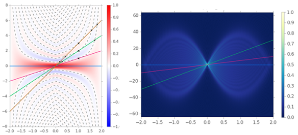
The following figures plot the AF of the one dimensional rectangular pupil and variation of OTF with focus error $W_{20}$ . In each figure, the plot on the left shows the ambiguity function and several lines corresponding to different defocus error $W_{20}$ . The zero value locai, $y = n/(2 - |u|)$ are denoted by the gray dashed lines. The intersection of zero value locai with the line(s) $y = 2uW_{20}/\lambda$ , which in the OTF plot represents the frequencies where the OTF is zero, is shown by the cross (‘x’) markers. The plots on the right show the corresponding variation of the OTF with different.

def plot_1dRectAF(w20LambdaBy2, N=15, umin=-2, umax=2, ymin=-8, ymax=8):
    """rudimentary function to show the AF

    Parameters
    ----------
    w20LambdaBy2 : list of real values
        specifies the amount defocus error W_{20} in
        terms of lambda/2. The slope of the OTF 
        associated with W_{20} in AF plane is 2*W20/lambda.
    N : integer
        number of zero value loci to plot 
    """
    u = np.linspace(umin, umax, 200)
    y = np.linspace(ymin, ymax, 400)
    uu, yy = np.meshgrid(u, y) # grid

    # Numpy's normalized sinc function = sin(pi*x)/(pi*x)
    af = (1 - np.abs(uu)/2)*np.sinc(yy*(2 - np.abs(uu)))
    # plot
    fig = plt.figure(figsize=(12, 7))
    ax1 = fig.add_axes([0.12, 0, 0.42, 1.0]) # [*left*, *bottom*, *width*,*height*]
    ax2 = fig.add_axes([0.6, 0.12, 0.38, 0.76])
    im = ax1.imshow(af, cmap=cm.bwr, origin='lower', 
                   extent=[umin, umax, ymin, ymax], 
                   vmin=-1.0, vmax=1.0, aspect=2./6)
    plt.colorbar(im, ax=ax1, shrink=0.77, aspect=35)
    # zero value loci
    for n in range(1, N+1):
        zvl = n/(2.0 - abs(u[1:-1]))
        ax1.plot(u[1:-1], zvl, color='#888888', 
                linestyle='dashed')
        ax1.plot(u[1:-1], -zvl, color='#888888', 
            linestyle='dashed')
    # OTF line on AF plane
    for elem in w20LambdaBy2:
        otfY = elem*u # OTF line in AF with slope 2w_{20}/lambda
        ax1.plot(u, otfY)
    # intersections
    def get_intersections(b): 
        # b is tan(phi) or 2w_{20}/lambda
        n = np.linspace(1, np.floor(b), np.floor(b))
        u1 = 1 + np.sqrt(1 - n/b)
        u2 = 1 - np.sqrt(1 - n/b)
        y1 = u1*b
        y2 = u2*b
        u = np.hstack((u1, u2))
        y = np.hstack((y1, y2))
        return u, y
    for elem in w20LambdaBy2:
        intersectionsU, intersectionsY = get_intersections(elem)
        ax1.scatter(intersectionsU, intersectionsY,
                    marker='x', c='k', zorder=20)

    # OTF plots
    for elem in w20LambdaBy2:
        otf = (1 - np.abs(u)/2)*np.sinc(elem*u*(2 - np.abs(u)))
        ax2.plot(u, otf, label='$W_{20}' + '= {}lambda/2$'.format(elem))
    # axis settings
    ax1.set_xlim(umin, umax)
    ax1.set_ylim(ymin, ymax)
    ax1.set_title('2-D AF of 1-D rect pupil P(x)', y=1.01)
    ax1.set_xlabel('u', fontsize=14)
    ax1.set_ylabel('y', fontsize=14)
    ax2.axhline(y=0, xmin=-2, xmax=2, color='#888888',
                zorder=0, linestyle='dashed')
    ax2.grid(axis='x')
    ax2.legend(fontsize=12)
    ax2.set_xlim(-2, 2); ax2.set_ylim(-0.2, 1.005)
    ax2.set_title("Optical Transfer Function", y=1.02)
    ax2.set_xlabel("u (scaled saptial frequency)", fontsize=14)
    #fig.tight_layout()
    plt.show()

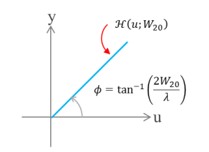
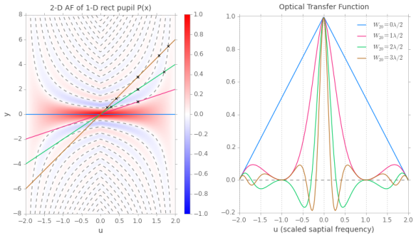
Plots of AF and OTF for which $W_{20} = n\frac{\lambda}{2}$ for $n=0, 1, 2, 3, \dots$ , i.e. $n \in \mathbb{Z}$ . The equation for the OTF was obtained directly from the ambiguity function by replacing $y$ with $2uW_{20}/\lambda$ .

The points of intersection between lines $y = 2uW_{20}/\lambda$ and each zero loci curve $y = n/(2 - |u|)$ (for $n > 0$ ) can be found by equating $n/(2 - |u|) = 2uW_{20}/\lambda$ , which gives $u = 1 \pm \sqrt{1 -\frac{n \lambda}{2 W_{20}}}$

For example, the line $y=2u \frac{W_{20}}{\lambda}\Big|_{W_{20}=1\lambda/2}$ intersects the zero loci curve $y = \frac{n}{(2 - |u|)}\Big|_{n=1}$ at $u=1$ , the line $y=2u \frac{W_{20}}{\lambda}\Big|_{W_{20}=2\lambda/2}$ intersects the curve $y = \frac{n}{(2 - |u|)}\Big|_{n=1}$ at $u=1 \pm \sqrt{1 - 1/2}$ , and the curve $y = \frac{n}{(2 - |u|)}\Big|_{n=2}$ at $u=1$ , and so on. As we can see, there are odd number of intersections of the lines with the zero loci curves when the defocus error $W_{20}$ is an integer multiple of $\lambda/2$ . This corresponds to an odd number of zero-value OTF points in the OTF plots when the defocus error $W_{20}$ is an integer multiple of $\lambda/2$ .

Note that we only found the abscissa ( $u$ coordinates) for the intersection points above.

plot_1dRectAF(w20LambdaBy2=[0, 1, 2, 3])

Plots of AF and OTF for which $W_{20} = n\frac{\lambda}{2}$ for $n=0.5, 0.99, 1.4, 3.6, \dots$ , i.e. $n \in \mathbb{R}, n \notin \mathbb{Z}$ (the particular values were arbitrarily chosen, and the $W_{20}=0$ line is plotted for comparison). In this case we find that there are even number of intersections for each line with the zero-loci curves in the AF plot. Correspondingly there are even number of zero-value OTF points for each OTF with focus error $W_{20}=n\lambda/2$ for $n \in \mathbb{R}, n \notin \mathbb{Z}, n \neq 0$ .

plot_1dRectAF(w20LambdaBy2=[0, 0.5, 0.99, 1.5, 3.6])

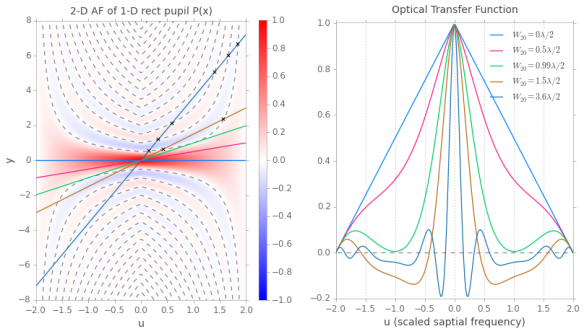
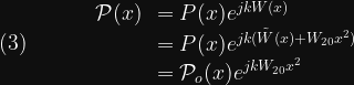
Also, note from the above plots that the first occurrence of the OTF intersecting/crossing the zero value happens as $W_{20} \to \lambda/2$ . This point is also the known as the traditional or Hopkins criterion for misfocus [4].

Example: Ambiguity function of cubic phase mask

Cubic phase masks (CPM) has been used to make hybrid optical systems largely invariant to defocus, thus extending the depth of field of such systems. For details on CPM systems, refer to [4].

The expression for the ambiguity function of a cubic phase mask is given below [4]:

$(14) \hspace{40pt} A(u, y) = \frac{1}{2} \int\limits_{-(1 - |u|/2)}^{(1 - |u|/2)} e^{j\alpha[(t+u/2)^\gamma - (t-u/2)^\gamma]}e^{j2\pi y t} dt, \hspace{10pt} |u| \leq 2;$

We will numerically evaluation the above expression for the AF of cubic phase mask (CPM), recognizing that the expression is of the form of inverse Fourier Transform of $g_u(t)$ where,

$g_u(t) = \frac{1}{2} e^{j\alpha[(t+u/2)^\gamma - (t-u/2)^\gamma]}$

Here are the steps for rendering the 2-D AF for CPM:

Create a $u$ vector $-2 \leq u \leq 2$
Create a $t$ vector $-2 \leq t \leq 2$ (i.e. between $-a-L \leq t \leq a + L$ , which is the maximum region of integration)
For every “u” in $u$ create the sequence $g_u(t)$ where, $g_u(t) = f(t + u/2)f^{*}(t - u/2)$ using the following rule:

a. if $-1 < u/2 < 0$ , then evaluate $g_u(t)$ where $-u/2 -1 < t < u/2 + 1$

b. if $0 < u/2 < 1$ , then evaluate $g_u(t)$ where $u/2 -1 < t < -u/2 + 1$
Take inverse Fourier Transform of each sequence $g_u(t)$ (with $y$ as the transform variable). i.e. $G_u(y) =$ $A(u,y) =$ IFFT $\{g_u(t)\}$

The expression for the OTF for the CPM is then given by:

$(15) \hspace{40pt} \mathcal{H}(u, W_{20}) = A(u, 2uW_{20}/\lambda) = \frac{1}{2} \int\limits_{-(1 - |u|/2)}^{(1 - |u|/2)} e^{j\alpha[(t+u/2)^\gamma - (t-u/2)^\gamma]}e^{j2\pi \left(\frac{2uW_{20}}{\lambda} \right) t} dt, \hspace{10pt} |u| \leq 2;$

We will use numerical integration to generate the plots of OTFs for the CPM with various amounts of defocus.

from scipy.integrate import quad
import warnings
warnings.simplefilter(action='error', category=np.ComplexWarning)
# Turn on the warning to ensure that the numerical integration is "reliable"?
warnings.simplefilter(action='always', category=sp.integrate.IntegrationWarning)

ifft = np.fft.fft
fftshift = np.fft.fftshift
fftfreq = np.fft.fftfreq

# cubic phase mask parameters
alpha = 90
gamma = 3
umin, umax = -2, 2
ymin, ymax = -60, 60
w20LambdaBy2 = [0, 5, 15] # amounts of defocus in units of wavelength (by 2)

uVec = np.linspace(umin, umax, 300)
N = 512  # number of samples along "t" ... and for FFT
L = 1

def gut(t, alpha, gamma, u): 
    return 0.5*np.exp(1j*alpha*((t + u/2)**gamma - (t - u/2)**gamma))

guy = np.empty((N, len(uVec)))
#roi = np.empty((N, len(uVec))) # for debugging & seeing the region of integration
t = np.linspace(-2*L, 2*L, N)
dt = (4*L)/(N-1)

for i, u in enumerate(uVec):
    g = np.zeros_like(t, dtype='complex64')
    if -1 <= u/2.0 < 0:
        mask = (t > (-u/2 - 1))*(t < (u/2 + 1))
        #roi[:, i] = mask.astype('float32')
        g[mask] = gut(t[mask], alpha, gamma, u)
        guy[:, i] = np.abs(fftshift(ifft(g)))
    elif 0 <= u/2.0 <= 1:
        mask = (t > (u/2 - 1))*(t < (-u/2 + 1))
        #roi[:, i] = mask.astype('float32')
        g[mask] = gut(t[mask], alpha, gamma, u)
        guy[:, i] = np.abs(fftshift(ifft(g)))

# Normalize to make maximum value = 1
guyMax = np.max(np.abs(guy.flat))
guy = guy/guyMax

yindex = fftshift(fftfreq(N, dt))
ymin, ymax = yindex[0], yindex[-1]

fig = plt.figure(figsize=(12, 7))
ax1 = fig.add_axes([0.12, 0, 0.5, 1.0]) # [*left*, *bottom*, *width*,*height*]
ax2 = fig.add_axes([0.66, 0.23, 0.32, 0.54])

im = ax1.imshow(guy**0.8, cmap=cm.YlGnBu_r, origin='lower',
               extent=[umin, umax, ymin, ymax],
               vmin=0.0, vmax=1.0,aspect=1./40)  
plt.colorbar(im, ax=ax1, shrink=0.55, aspect=35)

# OTF line in AF 
for elem in w20LambdaBy2:
    otfY = elem*uVec # OTF line in AF with slope 2w_{20}/lambda
    ax1.plot(uVec, otfY, alpha = 0.6, linestyle='solid')

ax1.set_xlim(umin, umax)
ax1.set_ylim(ymin, ymax)
ax1.set_xlabel('u', fontsize=14)
ax1.set_ylabel('y', fontsize=14)
ax1.set_title('2-D AF of 1-D cpm', y=1.01)

# Magnitude plots of the OTF of the cpm

def otf_cpm(t, alpha, gamma, u, w20LamBy2): 
    return (0.5*np.exp(1j*alpha*((t + u/2)**gamma - (t - u/2)**gamma))
            *np.exp(1j*2*np.pi*u*w20LamBy2*t))

def complex_quad(func, a, b, **kwargs):
    """Compute numerical integration of complex function between
    limits a and b
    Adapted from the following SO post:
    stackoverflow.com/questions/5965583/use-scipy-integrate-quad-to-integrate-complex-numbers
    """
    def real_func(x, *args):
        if args:
            return sp.real(func(x, *args))
        else:
            return sp.real(func(x))
    def imag_func(x, *args):
        if args:
            return sp.imag(func(x, *args))
        else:
            return sp.imag(func(x))
    real_integral = quad(real_func, a, b, **kwargs)
    imag_integral = quad(imag_func, a, b, **kwargs)
    return (real_integral[0] + 1j*imag_integral[0], real_integral[1:], imag_integral[1:])

for elem in w20LambdaBy2:
    Huw = np.empty_like(uVec, dtype='complex64')
    for i, u in enumerate(uVec):
        if -1 <= u/2.0 < 0:
            Huw[i] = complex_quad(func=otf_cpm, a=-u/2 - 1, b=u/2 + 1, args=(alpha, gamma, u, elem))[0]
        elif 0 <= u/2.0 <= 1:
            Huw[i] = complex_quad(func=otf_cpm, a=u/2 - 1, b= -u/2 + 1, args=(alpha, gamma, u, elem))[0]
    HuwMax = np.max(np.abs(Huw))
    ax2.plot(uVec, np.abs(Huw)/HuwMax, label='$W_{20}' + '= {}lambda/2$'.format(elem))

ax2.legend(fontsize=12)
ax2.set_ylabel("Magnitude of OTF", fontsize=14)
ax2.set_xlabel("Spatial frequency, u", fontsize=14)
ax2.set_title('Optical Transfer Function of cpm', y=1.01)

plt.show()

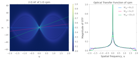
We can see from the above plots of the OTF, that the OTFs are insensitive to large amounts of defoucs. More importantly, there are no regions of zero values within the passband (though the bandwidth is not really constant for large amounts of defocus). This property is extremely important from the point of view of the reconstruction filter (such as an inverse filter or an Wiener filter).

References

Introduction to Fourier Optics, Joseph Goodman
The Ambiguity Function as a polar display of the OTF, K.H. Brenner, A.W. Lohmann and J. Ojeda-Castaneda, Optics Communication, 1982
Misfocus tolerance seen by simple inspection of the ambiguity function, H. Bartelt, J. Ojeda-Castaneda, and Enrique Sicre, Applied Optics, 1984.
Extended depth of field through wave-front coding, Edward R. Dowski, Jr., and W. Thomas Cathey, Applied Optics, 1995.

1 thought on “Ambiguity function (AF) and its use in OTF analysis”

Indranil Sinharoy on February 26, 2017 at 2:27 PM said:

I received a comment from Health Zhou via e-mail. He suggested that the line “rootsx =range(-8,0)+range(1,9)” should be change to “rootsx =np.hstack((range(-8,0),range(1,9)))”. I think, although it doesn’t change the code functionally, he has a fair point!.

Reply ↓

Indranil's world

Indranil's page on Imaging, Optics, Computer Vision, Python & Photography

Ambiguity function (AF) and its use in OTF analysis

The 2D Ambiguity Function (AF) and its relation to 1D Optical Transfer Function (OTF)

Example: Ambiguity function of a diffraction limited 1-D pupil.

Example: Ambiguity function of cubic phase mask

References

1 thought on “Ambiguity function (AF) and its use in OTF analysis”

Leave a Reply Cancel reply

The 2D Ambiguity Function (AF) and its relation to 1D Optical Transfer Function (OTF)

Example: Ambiguity function of a diffraction limited 1-D pupil.

Example: Ambiguity function of cubic phase mask

References

Rate this:

Let others know:

Like this:

1 thought on “Ambiguity function (AF) and its use in OTF analysis”

Leave a Reply Cancel reply