This is the third post in the series on Iris acquisition for biometrics. In the first and the second posts we saw that, at least in theory, iris recognition is an ideal biometric, and we went through some of the desirable properties of an iris acquisition system. However, currently most iris recognition systems require a single subject to stand (or move slowly) at a certain standoff distance from the camera in order capture and process iris images. Wouldn’t it be nice if iris recognition could be simultaneously performed for a group of people who may be standing/ moving within a large volume? Such systems could potentially be used in crowded places such as airports, stadiums, railway stations etc.

In this post, we will look at one of the limitations of current iris recognition systems – the limited depth of field, the fundamental cause of this limitation, and how some of the current systems are addressing this problem.

The problem of DOF

The inability of any conventional imaging system to capture sharp images within a large volume is illustrated in the Figure 1.

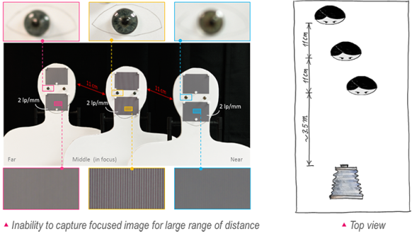
Figure 1 Depth of field (DOF) problem. Image of the three human-figure cut-outs with sinusoidal patterns (2 lp/mm) and artificial irises and placed apart by 11 cm from each other. The camera, with lens of 80 mm focal length and f/5 aperture, was focused on the middle cut-out (3.6 meters away from the camera). It is evident that the spatial resolution in the image falls off rapidly with increasing distance from the plane of sharp focus (middle cut-out) inhibiting the camera from resolving fine details uniformly across the imaging volume.

Perfect imaging corresponds to the ability of an imager to produce a scaled replica of an object in the image  space [1].  When only a small portion of the light  wave emerging  from an infinitesimally  small point source of light is collected through a finite opening of a camera’s aperture (Figure 2 (a)), the replica in the image space is not exact even in the absence of aberrations; instead, the image of the point spreads out in space due to diffraction at the aperture. This dispersed response in the three-dimensional image space is called Point Spread Function (PSF).  The spreading of the PSF along   the transverse (xy-axis) direction (a 2D PSF) restricts an imager’s ability to resolve fine details (spatial frequency) in the image. For an extended object, which is made of several points, the 2D PSF smears the responses from neighboring points into each other causing blur. Similarly, the spread along the longitudinal direction (z-axis) limits the ability to discriminate points staggered closely in the direction of the optical axis causing a region of uncertainty; however, the extension of the 3D PSF along the optical axis enables multiple spatially-separated objects (or points) within a volume in the object space to form acceptably sharp images at once.  Conversely, an (point) object in the object space may be placed anywhere within this zone and still form a satisfactory image. This zone of tolerance in the object space is called depth of field. The corresponding zone in the image space is called depth of focus [2]. In this post, the acronym “DOF” is used for both depth of field and depth of focus wherever its meaning is apparent from the context. In the image space, the DOF is defined as the region of the 3D PSF where the intensity is above 80% of the central maximum [3,4]. This zone is in the shape of a prolate spheroid. In the absence of aberrations, the maximum intensity occurs at the geometric focal point, , where contributions from all parts of the pupil are all in phase. Figure 2 (b) shows the aberration-free intensity distribution, , as a function of defocus  about the geometric focal point for a light source placed at 100 millimeters from a lens of focal-length of 25 mm and aperture diameter of 5 mm. The expression for the distribution—normalized to make  equal to unity—is obtained using scalar diffraction theory and paraxial assumptions.

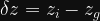
Figure 2 Incoherent impulse response and DOF. (a) The image A’ of a point source A spreads out in space forming a zone of tolerance called Depth of Focus (DOF) in the image space; (b) The normalized focal intensity distribution of the 3D PSF of a 25mm, f/5 lens imaging an axial point source at a distance of 100mm. The expression for the 3D PSF was obtained for a circular aperture using scalar diffraction theory and paraxial assumption. The DOF, having prolate spheroidal shape, is defined as the region within which the intensity has above 80% of the intensity at the geometric focus point. The figure shows iso-surfaces representing 0.8, 0.2, 0.05 and 0.01 intensity levels. The ticks on the left vertical side indicate the locations of the first zeroes of the Airy pattern in the focal plane. The vertical axis has been exaggerated by 10 times in order to improve the display of the distribution.

The shape—length and breadth—of the 80% intensity region (Figure 2(b)) dictates the quality of the image acquired by an imager in terms of lateral spatial resolution and DOF.

Continue reading →