In my last post, I described briefly how iris recognition works. I also described the four main modules that make up a general iris recognition system. In this post I am going to discuss some of the desirable properties of the iris acquisition module, or simply the iris camera. Although the acquisition module is the first block in the iris authentication/verification pipeline and it plays a very important role, the module has received much less attention of the researchers compared to the others.

Iris recognition algorithms have become quite mature and robust in past decade due to the rapid expansion of research both in industry and academia  [1–3]. Figure 1 shows a plot of the scientific publications (in English) on iris recognition between 1990 and 2013. The plot also shows the relative number of papers exclusively addressing the problems of the acquisition module, which is really very minuscule, compared to the total number of papers on iris recognition.

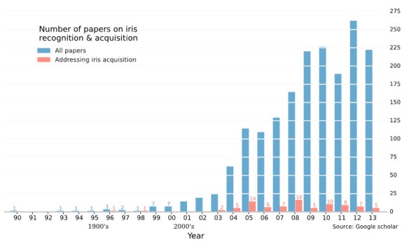
Figure 1. Number of publications in (English) journals on iris recognition between 1990 and 2013. The data was collected using Google scholar by searching the keywords IRIS + RECOGNITION + ACQUISITION + SEGMENTATION + NORMALIZATION + MATCHING. The plot shows that although the total number of research papers on iris recognition has grown tremendously during the last decade, the problems associated with iris acquisition have been overlooked.

The accuracy of iris recognition is highly dependent on the quality of iris images captured by the acquisition module. The key design constraints of the acquisition system are spatial resolution, standoff distance (the distance between the front of the lens and the subject), capture volume, subject motion, subject gaze direction and ambient environment [4]. Perhaps the most important of these are spatial resolution, standoff distance, and capture volume. They are described in details in the following paragraphs.

Two types of spatial resolutions are associated with digital imaging systems: the optical resolution, , of the lens, and the pixel (or sensor) resolution, , of the digital sensor.

For the purpose of this work, the optical resolution is defined as the maximum spatial frequency (present) in an object being imaged that can be resolved by the optics at a predetermined contrast [5]. In other words, it is a measure of the ability of an imager to resolve fine details present on the object surface. The optical resolution is governed by diffraction, and the deviation of a lens from ideal behavior, called aberrations. The resolution at the image plane of an aberration-free (also known as diffraction-limited) lens with Entrance Pupil Diameter (EPD), , and focal-length, , is given by [6]:

Where  is the F-number and  is the illumination wavelength. The entrance pupil is the image of the limiting aperture of the optical system as seen from object side through the lens elements in front of the limiting aperture. The optical resolution is measured in cycles per unit-length, typically cycles/mm or line-pairs-per-mm (lp/mm). The ISO/IEC 19794-6 [7] standards proposal for MTF recommends iris acquisition devices to maintain a minimum resolution of 2 lp/mm at the object with at 60% contrast [8]. Figure 2 plots resolution (maximum spatial frequency) against F-number for several contrast values calculated at the image plane for an illumination wavelength of 850 nm. The resolution in the object space is obtained as the product of the image plane resolution and the system magnification. For example, the magnification of a 100 mm focal length, F/4 camera at a standoff distance of 5 meters is about 0.02. If there are no aberrations, the resolution in the image plane at 60% MTF is 100 lp/mm (the value of red curve at F-number = 4 in Figure 2). The corresponding resolution in the object plane is 100 lp/mm x 0.02 = 2 lp/mm.

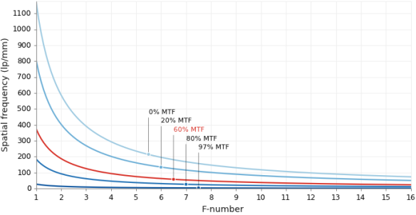
Figure 2. Maximum optical spatial frequency vs. F-number for different modulation transfer functions calculated for a wavelength of 850 mm at the image plane. The 0% MTF curve corresponds to the diffraction limited cutoff frequency for different F-numbers.

The sensor resolution is determined by the pixel density of the sensor. The ISO/IEC 19794-6 [7] standard requires at least 100 pixels across the iris diameter. Additionally, it recommends a pixel resolution of 200 pixels across the iris diameter [4,9]. For a digital sensor with pixel width  mm, the sensor Nyquist frequency is [10]:

The specified number of pixels across the iris diameter also determines the minimum required lateral magnification of the acquisition module [8].

As suggested earlier, large standoff iris recognition systems are highly desirable. Capturing high quality iris images at large distances is a difficult task [4,11]. Increasing the standoff distance while maintaining the pixel count (pixel resolution) on the iris requires the use of higher magnification (higher focal-length) optics as shown in Figure 3. However, arbitrarily increasing the focal-length to form an iris image of 200 pixels does not guarantee adequate optical resolution – an issue that has seldom been discussed in iris recognition literature. Once sufficient sampling has been achieved—either by using high pixel density sensor or through high magnification—the optical resolution ultimately dictates the image quality and consequently has a direct impact on the performance of iris recognition algorithms. As was shown by Ernst Abbe in his treatise on optical imaging, the diffraction limited optical resolution is independent of magnification and is solely determined by the F-number [12]. Increasing focal length of the system leads to loss of optical resolution as indicated by equation (1), unless the lens diameter is increased proportionally to maintain constant F-number (i.e. the F-number is not increased). However, smaller F-number lenses with larger focal lengths tend to be bulky and costly due to the use of larger number of optical elements required to correct for aberrations that scales with lens size [13]. Clearly, increasing the standoff distance from a few centimeters to a few meters without significant loss of spatial resolution is a challenge [14] for the iris recognition systems.

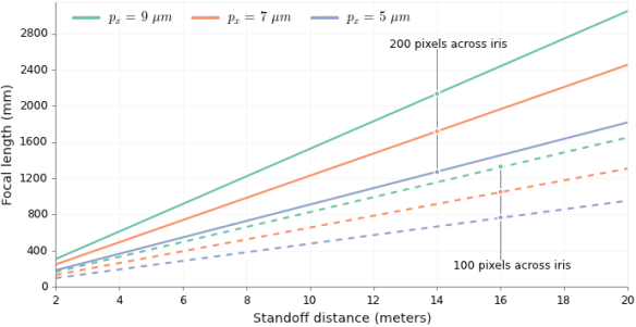
Figure 3. Focal length vs. standoff distance for maintaining 200 pixels (or 100 pixels represented by the dashed lines) across the iris for different pixel pitches.

For the purpose of the iris recognition task, the Depth of Field (DOF) of the iris acquisition system may be defined as a range of object distances within which the spatial resolution required for successful iris recognition is maintained above a predetermined threshold SNR [15]. Incorporating the requirement as specified by the ISO/IEC 19794-6 standard, this would mean that the DOF is the region of object distances where a spatial resolution of at least 2 lp/mm is with 60% contrast ratio is maintained. The most frequently employed definition of DOF in iris acquisition literature, which is derived from geometric optic, is:

Where,  is the focal-length,  is the F-number,  is the standoff distance, and , the circle of confusion, is a parameter that determines the smallest resolvable feature on the image of an object within the DOF. It is specified by the dimension of the blur spot in the image plane beyond which a point image is ruled out-of-focus [8]. A plot of the variation of the geometrically defined DOF with respect to the system F-number is shown in Figure 4. The geometrical DOF increases linearly with the F-number. However, DOF defined in within the framework of scalar diffraction theory (will be discussed in more details in the next post) is defined as the region near the geometrical focus where the intensity drops to 80% of the maximum intensity [16,17]. The diffraction based DOF is a function of the illumination wavelength and varies with the square of the F-number. In the image space it is given as:

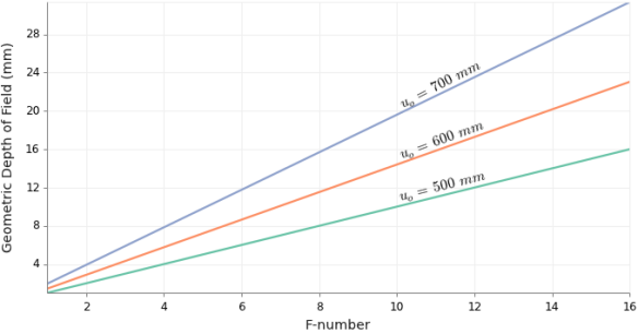
Figure 4. Geometric depth-of-field vs. system F-number (F#) for various object distances. The geometric DOF linearly increases with the F-number. The lens is assumed to have a 50 mm focal length, and the sensor has a pixel width of 5 microns.

Figure 5 shows the variation of the diffraction based DOF with respect to the F-number for different object distances.

The capture volume is generally referred to the three-dimensional spatial volume in which the user’s eye must be placed in order to acquire an iris image of predetermined quality [4,8,18]. The lateral extents (measured perpendicular to the optical axis) of the capture volume is determined by the FOV of the camera (provided it has sufficient resolution in the entire FOV), and the axial extent (measured along the optical axis) is determined by the DOF [8] of the lens. Time may also be included as the fourth dimension of the capture volume [9] which specifies the length of time the iris must be placed within the spatial capture volume to reliably capture iris image of sufficient quality and avoid motion-blur. For multi-camera systems and systems mounted in pan-tilt units, the net FOV is the total angular extents observable by the acquisition system.

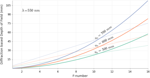
Figure 5. Diffraction depth-of-field vs. system F-number (F#) for various object distances. The diffraction based DOF, which are represented by the thick lines, increases proportionally with the square of the F-number. The lens is assumed to have a 50mm focal length, and the illumination wavelength is 550 nm. The thin plots are depict the variation of geometric DOF with F-number for 9 microns pixel size.

Currently, most commercially available iris recognition systems possess shallow DOF resulting in limited usability and increased system complexity [19]. Large capture volumes are not only desirable but also critical for making the iris recognition systems less constraining. Extending the zone of image capture will allow subjects to freely move, albeit while facing the camera, within this zone during the capture process. It will also allow multiple subjects to be identified/ verified simultaneously. Increasing the capture volume of current iris acquisition devices is expected to make biometric recognition easier to use and also make them commercially more feasible [20].

(The figures in the post were generated using Matplotlib, a Python based plotting library.)

Links to post in this series

1. Primer on iris recognition
2. *Desirable properties of iris acquisition systems
3. The DOF problem in iris acquisition systems

References

1. K. W. Bowyer, K. P. Hollingsworth, and P. J. Flynn, “A Survey of Iris Biometrics Research: 2008–2010,” in Handbook of Iris Recognition, M. J. Burge and K. W. Bowyer, eds., Advances in Computer Vision and Pattern Recognition (Springer London, 2013), pp. 15–54.
2. J. Daugman, “Iris Recognition,” in Handbook of Biometrics, A. K. Jain, P. Flynn, and A. A. Ross, eds. (Springer US, 2008), pp. 71–90.
3. A. Ross, “Iris recognition: The path forward,” Computer 43, 30–35 (2010).
4. J. R. Matey, D. Ackerman, J. Bergen, and M. Tinker, “Iris recognition in less constrained environments,” in Advances in Biometrics (Springer, 2008), pp. 107–131.
5. R. Narayanswamy, P. E. X. Silveira, H. Setty, V. P. Pauca, and J. van der Gracht, “Extended depth-of-field iris recognition system for a workstation environment,” in (2005), Vol. 5779, pp. 41–50.
6. J. W. Goodman, Introduction to Fourier Optics (Roberts & Co., 2005).
7. ISO/IEC 19794-6:2011, “Biometric data interchange formats — Part 6: Iris image data,” (2011).
8. D. A. Ackerman, “Optics of Iris Imaging Systems,” in Handbook of Iris Recognition, M. J. Burge and K. W. Bowyer, eds., Advances in Computer Vision and Pattern Recognition (Springer London, 2013), pp. 367–393.
9. J. R. Matey, O. Naroditsky, K. Hanna, R. Kolczynski, D. J. LoIacono, S. Mangru, M. Tinker, T. M. Zappia, and W. Y. Zhao, “Iris on the Move: Acquisition of Images for Iris Recognition in Less Constrained Environments,” Proc. IEEE 94, 1936–1947 (2006).
10. R. Jacobson, S. Ray, G. G. Attridge, and N. Axford, Manual of Photography (CRC Press, 2013).
11. C. Boehnen, C. Mann, D. Patlolla, and D. Barstow, “A standoff multimodal biometric system,” in Future of Instrumentation International Workshop (FIIW), 2011 (2011), pp. 110–113.
12. H. Gross, W. Singer, and M. Totzeck, Handbook of Optical Systems: Physical Image Formation (Wiley-VCH, 2005).
13. A. W. Lohmann, “Scaling laws for lens systems,” Appl. Opt. 28, 4996–4998 (1989).
14. L. Birgale and M. Kokare, “Recent Trends in Iris Recognition,” in Pattern Recognition, Machine Intelligence and Biometrics (Springer, 2011), pp. 785–796.
15. R. Narayanswamy and P. E. X. Silveira, “Iris recognition at a distance with expanded imaging volume,” in (2006), Vol. 6202, p. 62020G–62020G–12.
16. M., Bhatia, Avadh Behari, Wolf, Emil Born, Principles of Optics: Electromagnetic Theory of Propagation, Interference and Diffraction of Light(Cambridge Univ. Press, 2010).
17. H. Gross, Handbook of Optical Systems: Aberration Theory and Correction of Optical Systems (Wiley-VCH, 2007).
18. J. R. Matey and L. R. Kennell, “Iris recognition–beyond one meter,” in Handbook of Remote Biometrics (Springer, 2009), pp. 23–59.
19. R. J. Plemmons, M. Horvath, E. Leonhardt, V. P. Pauca, S. Prasad, S. B. Robinson, H. Setty, T. C. Torgersen, J. van der Gracht, and E. Dowski, “Computational imaging systems for iris recognition,” in Optical Science and Technology, the SPIE 49th Annual Meeting (2004), pp. 346–357.
20. R. Narayanswamy, G. E. Johnson, P. E. Silveira, and H. B. Wach, “Extending the imaging volume for biometric iris recognition,” Appl. Opt. 44, 701–712 (2005).