Thanks to the megapixel war, pixels in digital sensors have shrunk considerably over the years. Consequently, the pixel resolution (number of pixels in a digital image) has improved. Currently, the pixel resolution (assuming gray-scale sensor) can compete with the aerial resolution of lenses —on paper. This post is about a plot I created sometime back (for a different presentation) which shows the growth of pixel count and the diminishing of pixel size over the years for three popular segments of digital cameras. The green line plots the diffraction-limited (aberration free) optical resolution 3 stops below the maximum aperture available for off-the-shelf lenses during the same period. The optical resolution line doesn’t mean much; however, it is plotted to compare the sensor resolution with the optical resolution over time. The graph shows that while the sensor resolution has improved by leaps and bounds, the optical resolution hasn’t. It is no surprise though, because the optical resolution, which is limited by the fundamental nature of light —diffraction. Improving the optical resolution by traditional means is very expensive, and results in bulky lenses. The time is just right for exploring computational methods for improving the system resolution of imaging systems.
![]()
Other interesting data-points in the graphs are:
1. The Kodak DSC460, based on a Nikon SLR, was one of the first digital cameras.
2. The Sharp J-SH04 was the cellphone with a camera.
The number of mega-pixels and the pixel resolution (decrease in pixel size) has increased rapidly for the cellphone and point-and-shoot cameras, probably driven by marketing rather than by picture quality. In the more professional segment, clearly the strategy has been different. This may be because of two main reasons — one, the image quality dictated by noise, color reproduction, low-light performance, etc are more important for these shooters, and two, building high-quality large lens is relatively more expensive.
 (1)
(1) ,
,  is the focal length, and
  is the
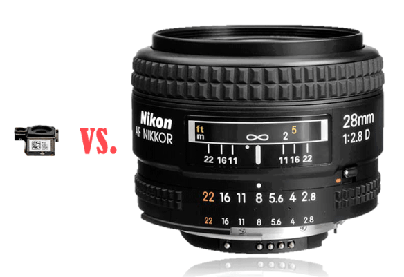
 , is the inverse of
  . The larger the value of
  , of a cellphone lens matches the
  times that of the DSLR lens. For example, a 50 mm, F/2.0 lens (D = 25 mm), which is a first order approximation of a 50 mm DSLR lens, can resolve details as fine as 54 microns focused at a distance of 2 meters. Whereas a 5 mm, F/2.0 lens (D = 2.5 mm), a close approximation of a typical cellphone camera lens, can resolve details only up to about 540 microns focused at the same distance. This is essentially a manifestation of the difference in magnifications (or angular resolution) of the lenses.